Moguls of Chaos with Deep Learning
After finishing my PyTorch certification on Coursera, I wanted to apply what I learned to a problem from physics, to get a feel for how data-driven models behave on a system I understand well. While looking for a model to train a neural network on, I remembered the toy model that Lorenz designed to show chaos in his book The Essence of Chaos: a sled going down a bumpy slope. I was curious to see if a trained neural network could predict the trajectories of the sleds and, ultimately, reproduce the same phase-space attractors as the physics-based model.
The code is in the repository. The model is introduced in Part 1, where I called it the “Moguls of Chaos”. Here I only recap it briefly, so I suggest reading that post first to get a feel for the dynamics and for how the sled version of the model is built.
Generating data
To train the neural network I generated sled trajecotories using the equations of motion. First of all, the slope with moguls is defined by
\[H(x,y) = -ax - b \, \cos(px) \, \cos(qy),\]where \(H\) is the height of the slope, \(a\) sets how steep it is (I use \(a = 0.25\), an angle of about 14°), \(b\) is the height of the bumps measured from the mean slope, and \(p\) and \(q\) are the spatial frequencies with which the bumps and pits alternate. I use \(p = 2\pi/10\) and \(q = 2\pi/4\), so the pattern repeats every 10 m downslope and every 4 m across the slope.
We drop a sled at the top of this slope, and because of the bumps, its trajectory bends as it makes its way down. The sled moves downslope at a constant speed \(u\), as if it had brakes and an engine to compensate for the pits and the bumps. This means that two sleds dropped at the same height, but separated by some distance, reach the bottom at the same time, even when their trajectories are very different. This assumption simplifies the dynamics a lot. The state of a sled is described by its downslope position \(x\) and velocity \(u\), and its cross-slope position \(y\) and velocity \(v\). But since \(u\) is constant, the downslope position is known at all times, \(x = x_0 + ut\), and only the cross-slope motion is left to compute. The equations of motion are
\[\frac{dy}{dt} = v, \qquad \frac{dv}{dt} = -F \, \partial_y H - c \, v,\]where \(c = 0.5\) s\(^{-1}\) is the friction coefficient and \(F\) is the force that keeps the sled on the surface of the slope,
\[F = \frac{g + H_{xx}u^2 + 2H_{xy}uv + H_{yy}v^2}{1 + H_x^2 + H_y^2},\]with \(g = 9.81\) m/s\(^2\). Written out, the derivatives of \(H\) are
\[\begin{aligned} H_x &= -a + bp \, \sin(px)\cos(qy), & H_y &= bq \, \cos(px)\sin(qy), \\ H_{xx} &= bp^2 \cos(px)\cos(qy), & H_{yy} &= bq^2 \cos(px)\cos(qy), \\ H_{xy} &= -bpq \, \sin(px)\sin(qy). \end{aligned}\]I generated the data by integrating these equations with a fourth-order Runge-Kutta solver (time step of 0.01 s), using \(b = 0.5\) m and \(u = 3.5\) m/s. All the sleds start at \(x = 0\), with \(y\) uniformly distributed in \([-L_y/2, L_y/2) = [-2, 2)\) m and the cross-slope velocity \(v\) uniformly distributed in \([-5, 5)\) m/s. I simulated 8000 sleds for 25 s, which is about 88 m down the slope. As in Part 1 the slope is a periodic tile, but here I keep \(y\) unwrapped, so every trajectory is a continuous curve, and I leave it to the network to deal with the periodicity (more on that below).
I split the data into a training set (80%), a validation set (10%) and a test set (10%). The split is done by sled, so no trajectory appears in more than one set.
Network
Inputs. The network takes five inputs: \(\sin(px)\) and \(\cos(px)\) for the downslope coordinate, \(\sin(qy)\) and \(\cos(qy)\) for the cross-slope coordinate, and the cross-slope velocity \(v\), divided by its standard deviation (about 1.9 m/s) so that all the inputs are of order one. The state of the sled is really just \((y, v)\), because \(x = ut\) is known. The downslope position works as a clock that tells the network where along the pattern of moguls the sled is.
Why sines and cosines? Because the slope is periodic, and for the network the dynamics should be periodic too. A sled that has wandered 20 m to the side finds exactly the same slope as the one inside the original tile. Since sine and cosine are bounded, the inputs stay between -1 and 1 no matter how far the sled wanders, and large values of \(y\) don’t bias the training. If I fed the raw \(x\) and \(y\) instead, the network would have to discover the periodicity by itself. (Note: I want to train the network on x and y values next and see what happens).
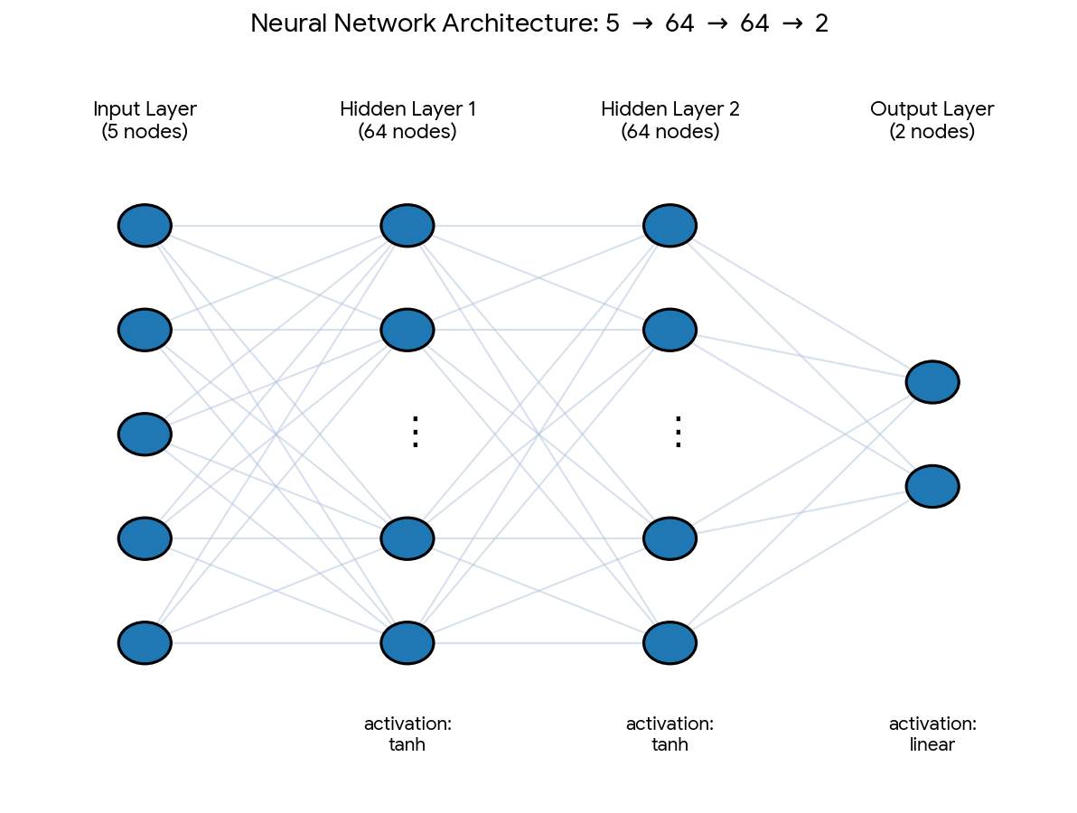
Architecture. It is a plain feed-forward network with two hidden layers of 64 neurons, each followed by a tanh activation, and a linear output layer with two neurons: \(5 \rightarrow 64 \rightarrow 64 \rightarrow 2\), which makes 4,674 trainable parameters. You can see a diagram of the architecture here:
Outputs. Instead of the next state, the network predicts the change of the state over a short time step \(h = 0.05\) s, that is, the vector \((\Delta y, \Delta v)\). For training, these changes are standardized (zero mean and unit standard deviation, computed from the training set).
Training. I cut every training trajectory into pairs: the state at one time (the five inputs) and the change over the following 0.05 s (the two outputs). With 6400 training sleds and 500 steps each, this gives 3.2 million examples. So during training the network only learns to predict a single step, and it never sees a whole trajectory. The loss function is the mean squared error between the predicted and the true changes, and I minimized it with the Adam optimizer, using a learning rate of 0.001 and mini-batches of 4096 examples. The computing time was fast, and the error kept going down as the epochs went by, so I trained the network for 20 epochs, where the error dropped to \(1e-4\). (This error is in standardized units, where 1 means that the network is no better than always predicting the average change.)
Predicting a trajectory. To predict a whole trajectory, I feed the network its own output. This is the forward algorithm:
- Start from the initial condition \((y_0, v_0)\) at \(x = 0\).
- At step \(n\), compute the downslope position \(x_n = u \, nh\) and build the five inputs from \(x_n\) and the current state \((y_n, v_n)\).
- The network returns the change \((\Delta y_n, \Delta v_n)\) over the next 0.05 s, which I rescale back to meters and meters per second.
- Update the state: \(y_{n+1} = y_n + \Delta y_n\) and \(v_{n+1} = v_n + \Delta v_n\).
- Repeat 500 times to cover the 25 s.
After the first step, the network never sees the true trajectory again, so its small errors are fed back as inputs. This is what makes the test demanding: the question is not whether the network predicts one step well, but whether its errors stay small over 500 steps.
Results
I picked the case \(b = 0.5\) m because, from Part 1, we know that the system is chaotic there: the bifurcation diagram shows chaotic solutions for bumps of 0.4 m or higher. This makes it a hard test, because in a chaotic system small errors grow quickly.
To demonstrate, I compare the trajectories of 7 sleds randomly selected from the test set, which the network never saw during training. The blue line is the true trajectory and the orange line is the one predicted by the network, which only received the initial condition at \(x = 0\).
What we can see is that in the first 10 m down the slope, the network matches the true trajectory pretty well. After about 20 m, for some sleds the predicted trajectory starts to diverge from the true one. This is probably because the system is chaotic: the network is only an approximation of the true dynamics, so it makes small errors at every step, and chaos amplifies them as the sled goes down. We saw the same mechanism in Part 1, where boards that started only 1 mm apart followed practically the same path for 20 m before they started to separate. For sleds 574 and 118, the predicted trajectory matches the true one all the way down. These sleds follow periodic trajectories, which don’t amplify small errors.
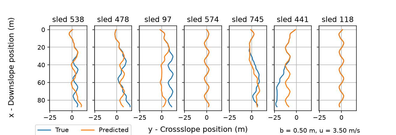
True (blue) and predicted (orange) trajectories of 7 randomly selected test sleds, for b = 0.5 m and u = 3.5 m/s. The network only receives the initial condition at x = 0 and then feeds on its own output. Each panel shows one sled going down the slope, and y is not wrapped, so the sleds can wander across several tiles.
To quantify how the predictions degrade as the sleds go down the slope, I computed the root mean square (RMS) error between the predicted and the true trajectories over all the test sleds, as a function of time.
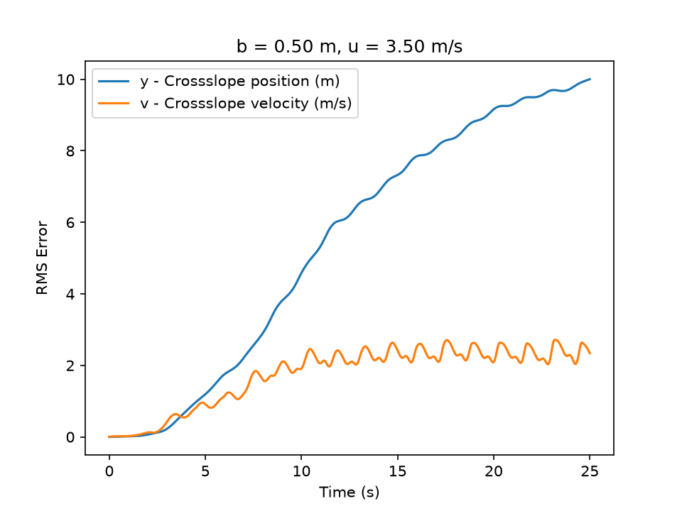
RMS error of the predicted cross-slope position y (blue) and velocity v (orange) as a function of time, computed over the test sleds for b = 0.5 m and u = 3.5 m/s. At 3.5 m/s, 5 s correspond to about 18 m down the slope and 10 s to 35 m.
The error is tiny at the beginning: during the first 3 s (about 10 m down the slope) the error in \(y\) stays below half a meter. Then it grows, reaching about 1 m after 5 s and about 5 m after 10 s. This quick growth has a flavor of chaos, and it agrees with what we saw in the individual trajectories, where the predictions started to separate after about 20 m. After 10 s the error in the velocity stops growing and fluctuates around 2 to 2.5 m/s, which is comparable to the spread of the velocities themselves (the friction keeps \(v\) bounded between -5 and 5 m/s). At that point the network doesn’t know the velocity of a particular sled anymore. The error in \(y\) keeps growing, but more slowly, until it reaches about 10 m at the end. Remember that \(y\) is not wrapped, so a sled that the network puts in the wrong lane counts as an error of several meters, and by the end of the run the sleds themselves are spread over about 10 m across the slope.
The network cannot follow an individual sled for more than 5 to 10 s, but that is what we expect from a chaotic system. In Part 1, a difference of 1 mm in the initial position was enough to make two boards go their separate ways, and any model that makes even tiny errors will drift away from the true trajectory after some time. What matters in the end is whether the network learned the dynamics well enough to produce the same attractor as the physics-based model. To check this, I compared the phase space of all the test sleds at different distances down the slope. The sleds are dropped at \(x = 0\) with \(y\) and \(v\) uniformly distributed, so they start as a uniform cloud that is stretched and folded as they go down the slope until the strange attractor appears.
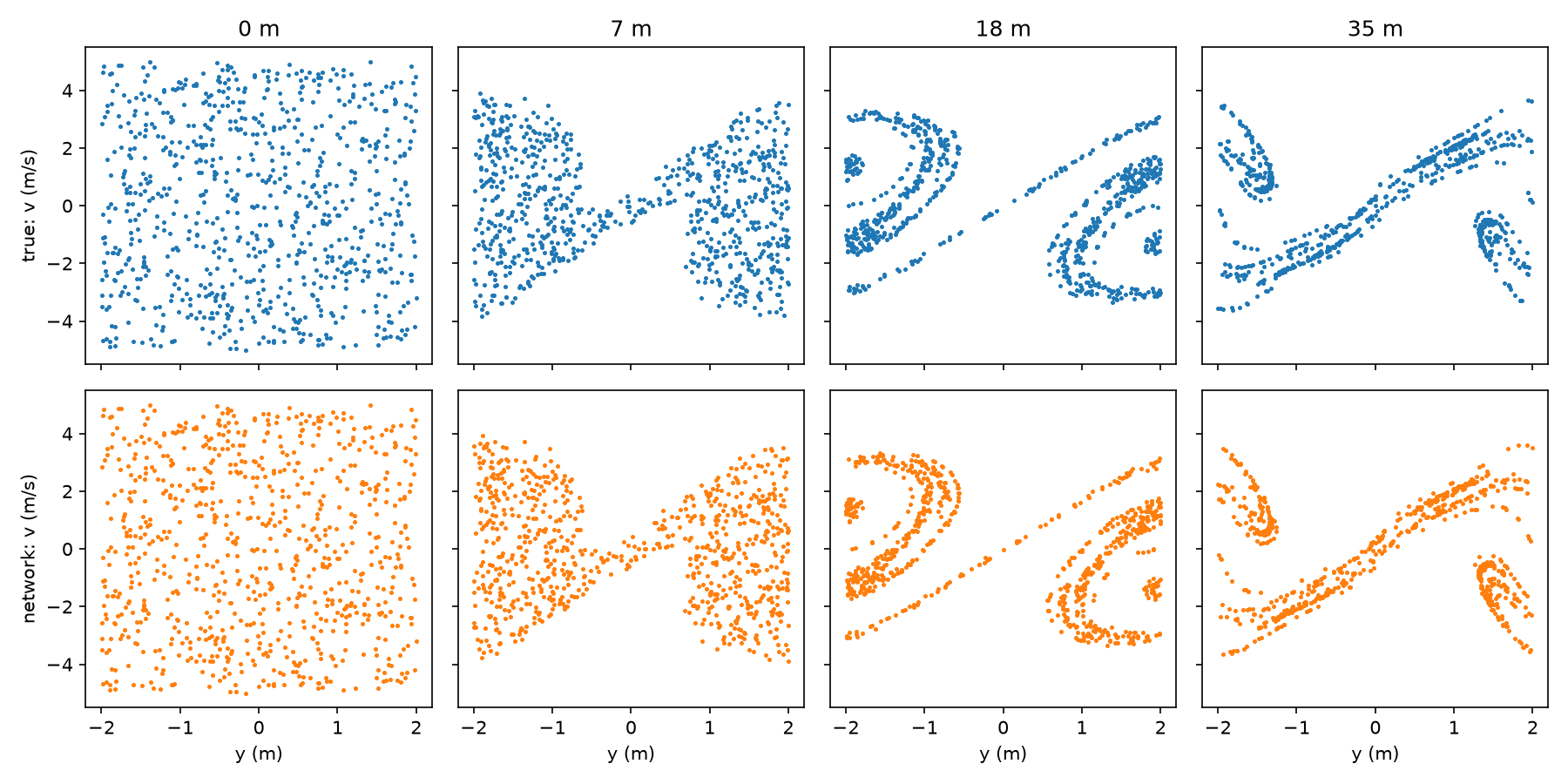
Phase space \((y, v)\) of the test sleds at 0, 7, 18 and 35 m down the slope (0, 2, 5 and 10 s). Top row: true (blue). Bottom row: predicted by the network (orange), which only receives the initial conditions at 0 m. For display, \(y\) is wrapped into the periodic tile \([-2, 2)\) m.
The top row shows the true phase space and the bottom row the one predicted by the network. At 0 m both are identical, by construction, because the network starts from the same initial conditions. The phase plots for the predicted sleds further down the slope manage to follow the same manifold as the true sled, but if you compare the true and predicted at the same down slope distance, there points are arranged differently, because the trajectories are different.
This is the part I find most interesting. At 35 m, 10 s after the start, the RMS error tells us that the individual predictions are already far off, about 5 m in \(y\) and 2 m/s in \(v\). The individual points no longer sit in the same places, yet the predicted cloud is distributed on the same attractor. In other words, the network did not learn to follow each sled, but it did learn the dynamics that shape the attractor: the stretching and folding that all the sleds go through.
Here is the same comparison as an animation, as the sleds go down the slope:
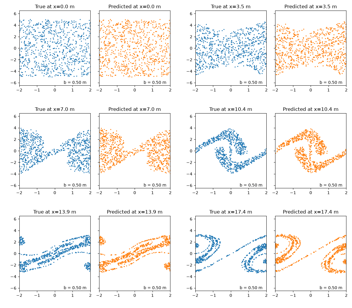
Animation of the phase space \((y, v)\) of the test sleds as they go down the slope, for b = 0.5 m and u = 3.5 m/s. True (blue) and predicted by the network (orange).
I’m thinking of doing the same but on an aperiodic bumpy slope. I wonder if the network will struggle representing the physics. If it doesn’t, it might be a nice to implement some physics into the network.