Moguls of Chaos
What are the moguls and why are they related to chaos? Mogul skiing is a ski discipline that consists of descending a slope full of small regular bumps, where the skills and technique of skiers are tested to its full. Ed Lorenz, an outdoorsman and science legend, discovered that objects descending the moguls exhibit chaotic behavior. He built a small numerical model to explore the dynamics of an idealized board descending such type of slopes and exemplified some of the tools used for characterizing chaos.
This project aims to perform the small numerical experiment that Ed did and explained in his book The Essence of Chaos, to show how we can construct parsimonious models that exhibit chaos from real case phenomena.
I started this small project two years ago after reading the above-mentioned book, but I couldn’t finish it, and given that I am required to do a small project for my scientific computing class, I will use it as an opportunity to finish once and for all this mini-project. Also, this problem is an excuse to refresh my very rusty Julia skills and to keep my Python skills sharp. This post doesn’t show the code used to solve the equations or plot the examples, but it can be found in the following repository.
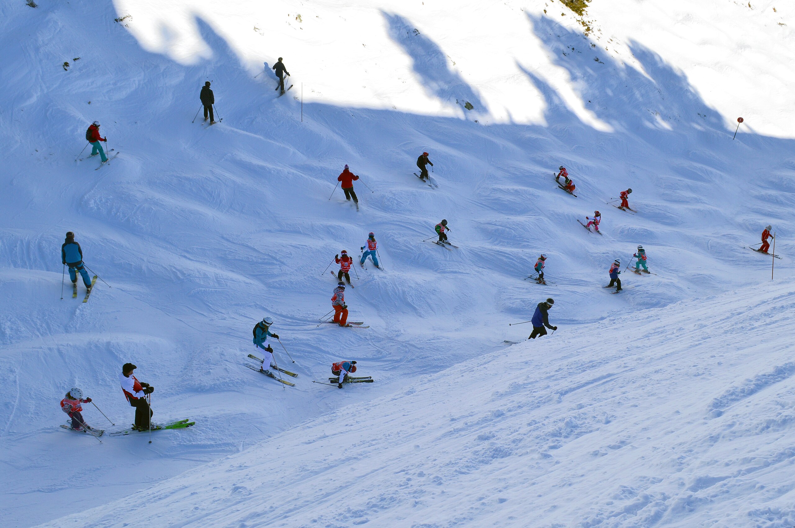
Ski school on moguls, Edelweiss slope, Les Arcs. Photo by DimiTalen - Own work, CC0, https://commons.wikimedia.org/w/index.php?curid=125707415.
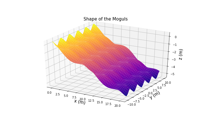
The ski slope model consists of a board that goes down a regularly-bumpy slope or moguls without any control of the direction whatsoever. The dynamical system of this board is described by the system of ODEs shown bellow.
\[\frac{dx}{dt} = u, \quad \frac{dx}{dt} = v, \quad \frac{dz}{dt} = w.\]\begin{align} \frac{du}{dt} &= -F \partial_x H - cu, \end{align} \begin{align} \frac{dv}{dt} &= -F \partial_y H - cv, \end{align} \begin{align} \frac{dw}{dt} &= -g + F - cw, \end{align}
where \(\vec{x} = (x,y,z)\) are the spacial coordinates and \(\vec{u} = (u,v,w)\) are the components of the velocity of the board. \(H\) is the shape of the slope that is parameterized by the following expression:
\[H(x,y) = -ax - b \ cos(px) \ cos(qy),\]where \(p\) and \(q\) are the spatial frequencies in which the bumps and pits alternate. The \(a\) parameter is the angle of the slope and the \(b\) parameter can be seen as the height of the bumps measured form the mean slope (remember this parameter because it will be important for the last section).
This system of equations can be solved numerically using a Runge-Kutta scheme, thus, our first objective is to integrate several solutions for different initial conditions to observe the behavior of the board.
Boards down the slope!
I used the fourth-order Runge-Kutta method as an integrator and wrap it around a solver, to integrate the four variables of the system. Once the solver is working properly, we can compute the solutions for different boards.
Example 1
For this example we set the initial conditions for ten boards, with slight variations in their initial position: \(x = 0.0\) m, \(u = 3.5\) m/s, \(v = 0\) m/s, and \(y\) it is randomly chosen form the interval \([0,1]\) m, in a way that \(y\) is different for every board. The resulting trajectories can be seeing int the following figure.
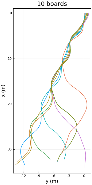
We can see how the boards follow similar trajectories, down until 10 m, where they start to diverge.
Example 2 We can explore the behavior with other initial conditions, but this time we set the \(y\) position of 7 boards only 1 mm apart between the values \([0.497, 0.503]\) m, keeping the same values for \(x,u,v\) used in the previous example.
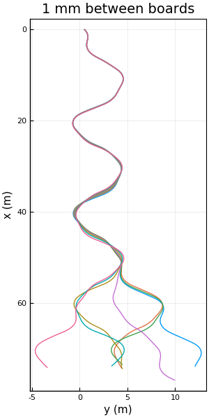
The figure above shows how the trajectories of the boards are practically the same until 20 m down the slope. After 20 m, some small variations appear in the trajectories of the boards, until they start growing bigger and bigger. Around 50 m down the slope, the trajectories diverge completely one from another, following very different paths.
These boards are a perfect example of a system that is sensitive to initial conditions, i.e. that small perturbations or variations in the initial conditions can lead to totally different solutions at some time in the future, which is commonly known as chaos.
From the trajectories of the boards is difficult to find regularities in the dynamics of this system, because the trajectories appear to behave randomly as they go down the slope. Therefore, in order to find regularity, we can use the velocities of the boards as they go down the slope. One of the tools that are very handy in the dynamical systems is the phase space plots, which basically consists of plotting the velocity of a system against its position. The problem is that our system has two spatial coordinates and two velocities components, which would make our phase space plot four-dimensional. Our brains can’t handle a four-dimensional space, so we need to do some modifications to our system in order to reduce its dimensions to only three.
Sleds down the slope!
To reduce the dimensions of our system, we can make the downslope velocity constant, or in the real world scenario, by equipping our board with some brakes and an engine so it can maintain a constant velocity while going down the pits or up the bumps, transforming it into a sled! In a mathematical sense, we say that \(\partial_t u = 0\). This modification allows us to neglect the \(u\) component of velocity and reduce the phase space to three dimensions.
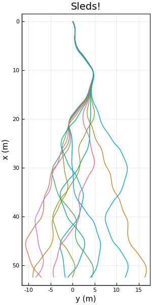
The previous figure shows eleven sleds going down the slope, with initial conditions \(x = 0\) m, \(y = [0, 0.1]\) m, \(v = 2\) m/s, and \(u = 3.5\) m/s. We see that the system behaves chaotically even though the downslope speed is maintained. We also see how all the sleds reach the same downslope position by the end of the simulation.
Sleds and strange attractors
Now our system has 3 variables, which will allow us to visualize its phase space plot. But the modifications that we need to do to our system are not over. If we see the trajectory-plots displayed above, we can see that \(x\) and \(y\) grow infinitely, which means that our phase space plot will not be compact, just a collection of points scattered around an infinite domain. The good news is that the cross-slope velocity is already bounded between \([-5, 5]\) m/s because of friction.
We need to find a way to make our system compact while preserving the physics of the system. If we analyze closely the structure of our mogul-slope, we can see that it is a collection of regular bumps and pits, that repeat themselves towards infinity.
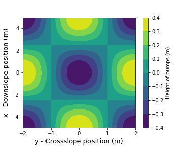
Therefore, we can crop our domain in a tile (figure below) from which we can reconstruct our full slope by placing consecutive tiles next to one another. In other words, we take this tile and set its boundaries to be periodic, so whatever exits the right side, re-enters the domain by the left side, and whatever exits the domain in by the lower boundary, re-enters by the top boundary. This slope-tile is defined in the domain: \(x \in [-5,5]\) m and \(y \in [-2,2]\) m.
The washing machine!
Once that our system is compact, we can run some simulations to plot the phase space of the system. The thing is that if we run it for one sled, we will see only a point traveling with apparent random motions in the 3D domain. So, a good idea would be to simulate a good amount of sleds, an ensemble of sleds, with the same downward velocity and with random initial positions (inside the domain of the tile) and random cross slope velocities. This will fill the phase-space of points and we will be able to see how they evolve as the descend the moguls. The downside of this is that it will be really difficult for us to identify any structures in the phase space because basically, the phase space plot will consist of a turbulent soup of points that flows down weirdly.
To cope with this visualization challenge, we can use another tool called Poincaré maps, in which we intersect the phase space with a plane transversal to the “flow”, which in our case are planes defined by \(x = \text{constant}\). However, we can take advantage of the feature that our sleds descend the slope with constant velocity \(u\) to define our version of the Poincaré map. In other words, we set the downward velocity of the ensemble to be the same for all the members, but with different cross-slope positions and velocities, in a manner that they will form planes that go down the slope. This set-up will allow us to get rid of the \(x\) coordinate in the phase space plot and only plot \(v\) against \(y\).
For the first run, we set an ensemble of 8000 sleds, all starting from \(x = 0\) m, but with random \(y\), random cross slope velocities \(v\) and with \(u = 3.5\) m/s, for all the members. The result can be seen in the following animation.
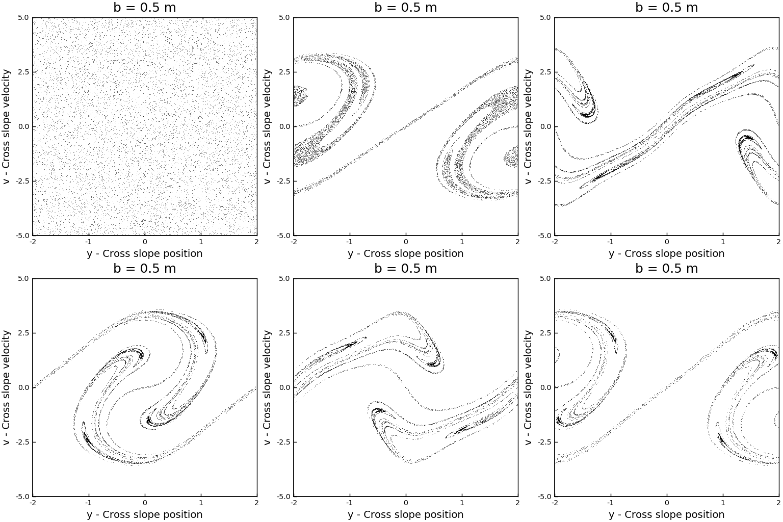
We can see that the corresponding strange attractor is like a horseshoe map. It reminds me of a washing machine!
Routes from Chaos
The bump height of the previous example was \(b = 0.5\) m, but what if we change this parameter to a smaller or bigger one? What will happen to the trajectories of the sled?
If we do a mental experiment and we set the height of the bumps to zero, we would have a plain slope without bumps and is easy to see that the trajectories of the sleds, in this case, would be straight (if \(v_0 = 0\)), therefore not chaotic. If we increase little by little the height of the bumps, we will start creating perturbations to the trajectories of the slopes, until the become chaotic, like in the previous case with \(b = 0.5\) m. So a better question to ask would be: when does it occur this transition from a non-chaotic system towards a chaotic one?
As a first approach to answer this question, we can perform a couple of simulations with different values of \(b\) to have an idea of the behavior of the system. Arbitrarily I selected the values for \(b\) to be \(0.11\) m, \(0.2\) m and \(0.66\) m. The phase space plots of these simulations can be seen in the following animation (where the one with \(b = 0.5\) m is also displayed).
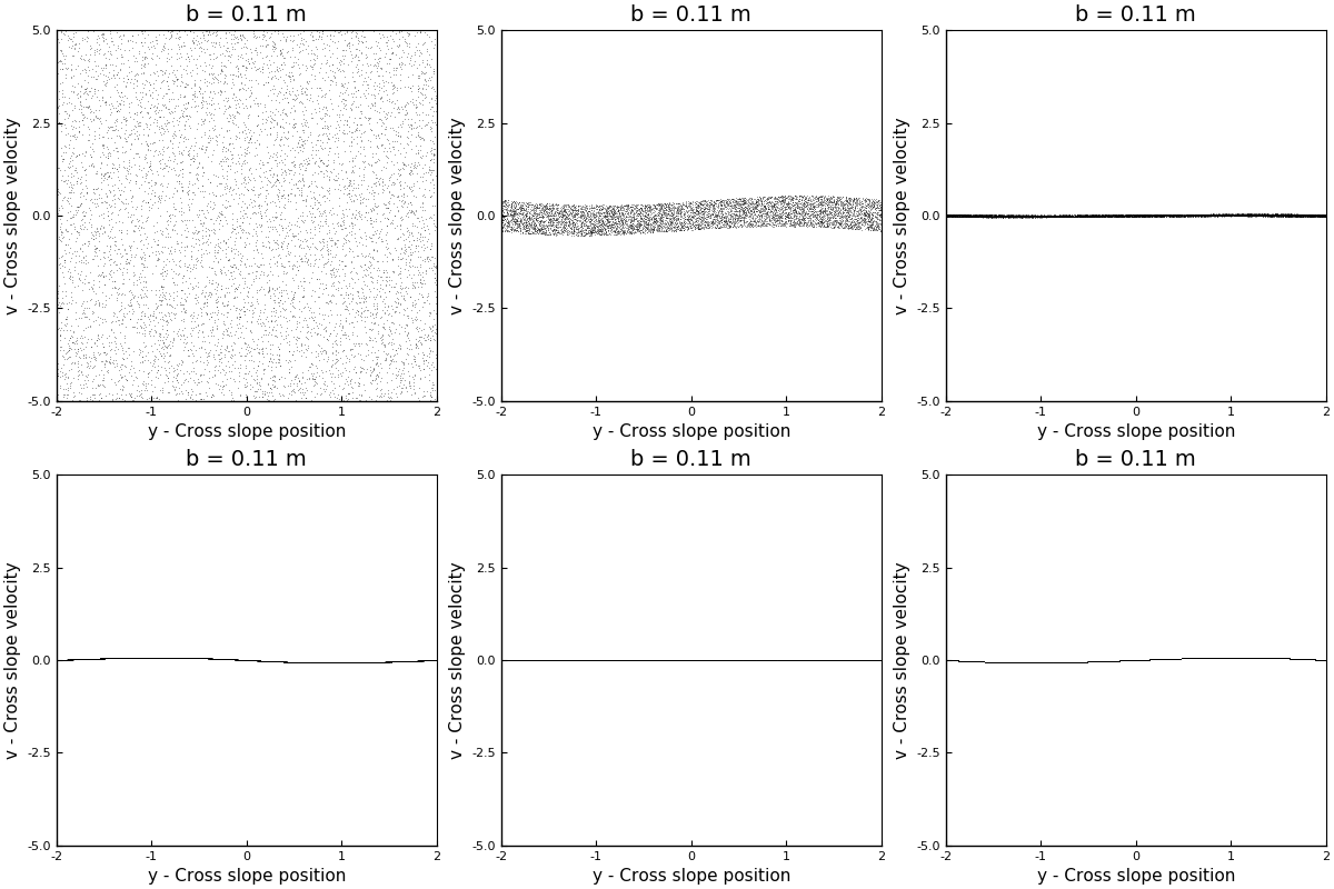
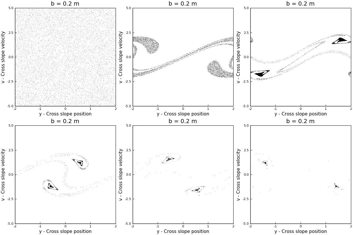

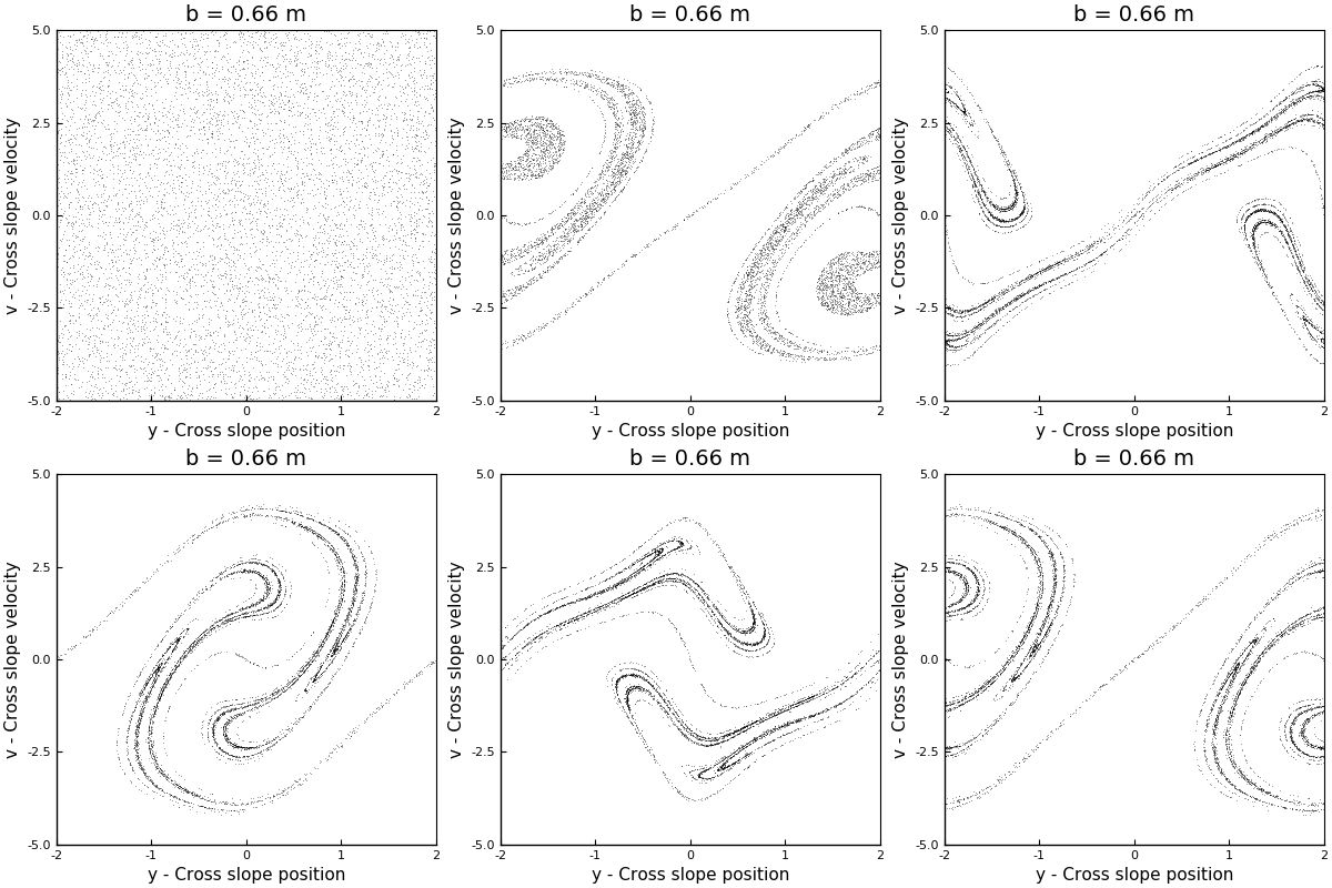
In the case with \(b = 0.11\) m, we can see how the points collapse to a line that oscillates like a standing wave, with a node at the center, and which has no signals of chaos. For \(b=0.2\) m, we can see more structure, but we see that as the sleds keep descending, the points collapse around two stable solutions. However, for \(b = 0.5\) m and \(b = 0.6\) m, we see the appearance of strange attractors, which shapes follow a loop that remains constant in time. From this runs, we can say that the firsts two cases don’t exhibit chaos, but the last two did. In other words, as \(b\) increases, the system becomes chaotic.
Bifurcation diagram
To answer the question of when the transition to chaos happens, we can construct something called bifurcation diagram, in which a variable of relevance is plotted against the parameter which forces the system to change its behavior. In our case, the forcing parameter is \(b\) the height of the bumps and the variable of relevance would be the cross-slope speed.
To produce the bifurcation diagram, we select an interval from \([0, 0.7]\) m for \(b\) with 7000 points, in which for each one of those b values, we perform a simulation for one sled for a long time, giving us 7000 solutions for different \(b\)s. For each one of these solutions, we need to remove the transient states, where the solution transitions towards its corresponding stable solution, if there is one. Keeping only the last steps of all the solutions, we are interested in plotting the cross-slope speed (the absolute value of the cross-slope velocity), but we are only interested in the local maximum values, i.e., when the sled changes the direction of movement. This is our indicator of periodicity in the solutions. If the sled has a periodic solution, it will have have the same local maximums as it goes down, but if its solution is not periodic, these changes of direction will be completely random.
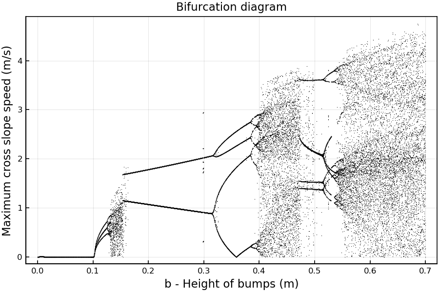
In the figure above we see the bifurcation diagram of our system. We observe that there are regions where there are lines and regions where there are clouds of points. The regions with clouds of points correspond to chaotic solutions where there is no periodicity of in the trajectories of the sled, and the regions where there are only lines indicate states in which the sled follow periodic trajectories.
From the bifurcation diagram, is possible to see that the system is periodic from \(b = 0\) m to \(b = 0.1\) m . Around \(b = 0.1\) m, a bifurcation occurs where apperently the system transitions into chaos (period three implies chaos), and then goes back to a periodic solution, from \(b = 0.15\) m to \(b = 0.4\) m. Finally, when the height of the bumps is \(b = 0.4\) m or greater, the sled trajectories are chaotic, with an apparent periodicity between \(b = 0.5\) m and \(b = 0.6\) m.
Returning to the question, we can fairly say that the transition to chaos happens then \(b = 0.4\) m, with some hiccups of chaos in the interval \(b = [0.1, 0.15]\) m.
Conclusion
I truly believe that this is a perfect example to show how it is possible to construct simple models from real case scenarios, and how a simple analysis can lead you to find some order and structure in the apparent chaos. After doing this mini-project, I feel more interested in applying these concepts to current research topics, where perhaps can be useful to throw some light into some undiscovered physics.
References
- Lorenz, Edward N. The Essence of Chaos. Univ. of Washington Press, 1993.
- Li, Tien-Yien, and James A. Yorke. Period three implies chaos. The American Mathematical Monthly 82.10 (1975): 985-992.