2D Simulation of Convection in a Stratified Fluid
The objective of this project was to study the effect of convection in a stratified fluid, trying to simulate the convection processes in the atmospheric boundary layer under a thermal inversion. For this, we performed a simulation using Dedalus, which is a Python framework used for solving PDEs using spectral methods. The simulation was performed to be compared with laboratory experiments done by Andrea Burgos, in which she used salinity gradients to set the stratification to simulate a thermal inversion.
For this particular simulation, we defined our domain using a Fourier and Chebyshev basis to solve the equations that describe the problem. In particular, we used a Fourier basis for the horizontal component and a Chebyshev basis for the vertical component, which allowed us to have periodic boundaries on the sides and fixed boundaries above and below the domain.
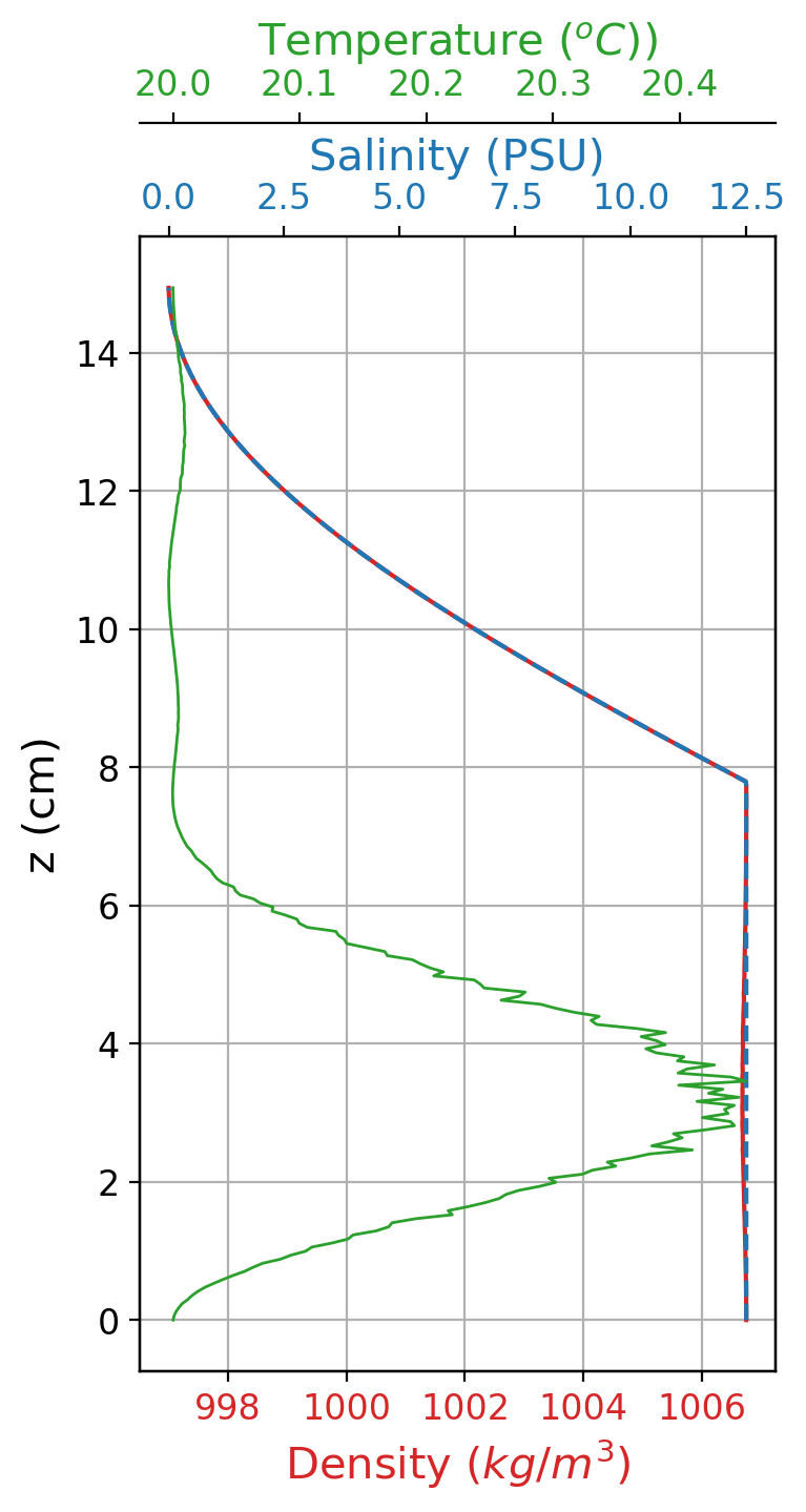
The stratification profile in the simulation was established using salinity gradients (as shown in the figure below) in such a way that the domain had a larger density in the lower half of the domain, and started diminishing linearly as height increased in the upper half of the domain. The initial temperature profile was set to 20ºC for the entire domain, with some noise added in the lower part of the domain to help initiate convection. The upper boundary condition for the temperature was set to 20ºC and the lower boundary condition was set to 28ºC.

Results
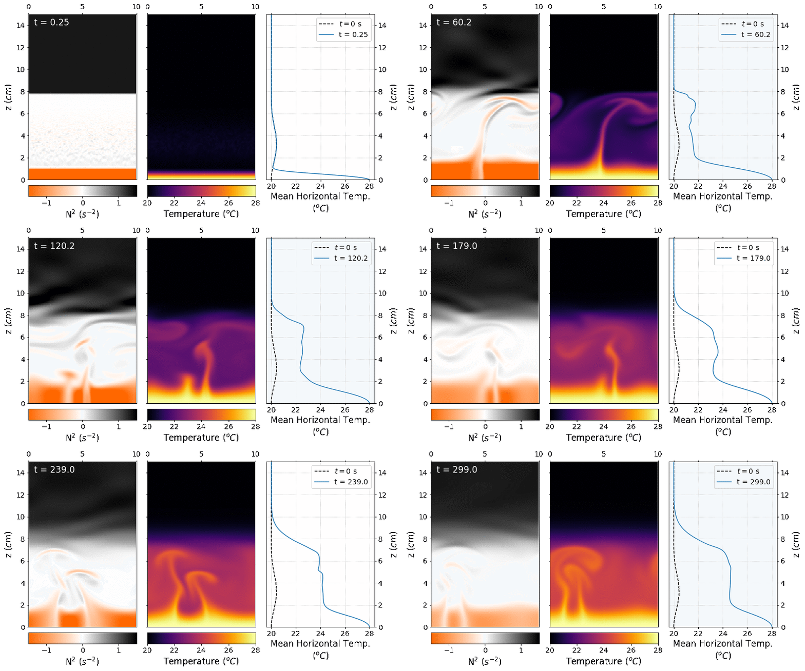
The domain dimensions used were 256 x 256 points, and the simulated time was 300 seconds, which took around four hours, using 8 cores. The final simulation can be seen in the following animation. The left panel shows the squared Brunt-Väisälä frequency which is an indicator of the stability of the fluid parcels (if \(N^2>0\) is stable and if \(N^2<0\) is unstable). The center panel shows the temperature field, and the right panel the evolution of the mean horizontal temperature profile.

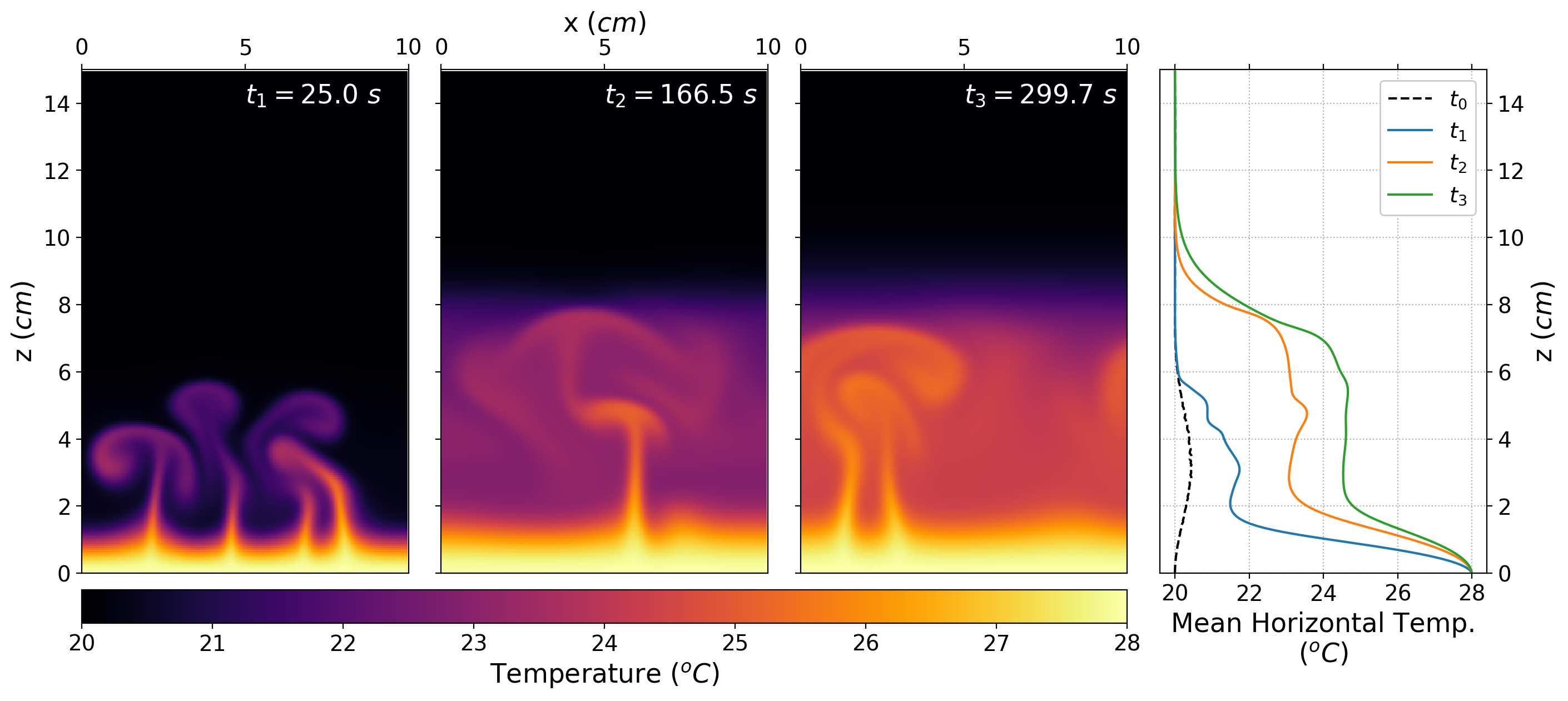
The picture below shows some snapshots of the temperature field at different times with their respective mean horizontal temperature profiles in the right panel. We can see how the bottom half of the domain starts to heat while the upper half it remains at 20ºC and at the interface it gradually increases the temperature. The hot plumes are unable to break the stratification and they remain trapped in the bottom half.

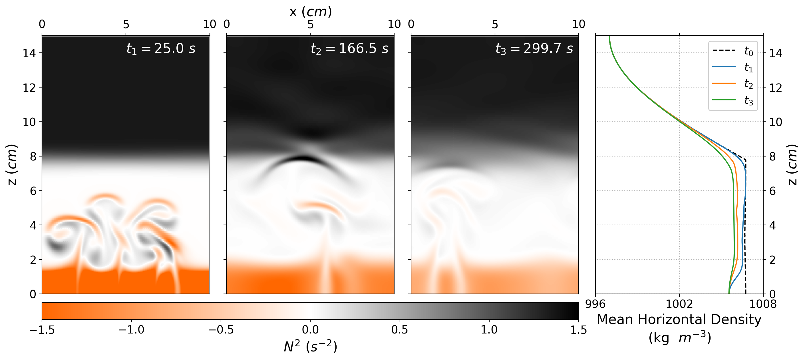
The following figure shows some snapshots of the squared Brunt-Väisälä frequency and the corresponding density profile in the right panel. We can see how the layer that is in contact with the bottom boundary is unstable the layers above it are neutral and stable. The convection plumes are unable to break the stratification profile above them because their density remains greater than that of the upper layer, i.e., the density variation set by the salinity is stronger than the density changes of the temperature. In the interface, the density decreases by 2 \(kg/m^3\), which indicates that there is some mixing in this region. Although, the mixing between the bottom and the upper half remains small after 300 seconds of simulation.

You can find the video in Youtube in the following link.
Acknowledgments
Thanks to Andrea Burgos and Angel Ruiz-Angulo for their help and support in doing this project. I had a great time in the Lab!
This work was part of my bachelor’s internship done at the Laboratory of Geophysical Fluid Dynamics, at the Center of Atmospheric Sciences UNAM. The results were presented in a poster in the Annual Mexican Geophysical Union in 2017, in Puerto Vallarta.